ST117 Lab 9

Linear regression, Model diagnostics

Author

Mengqi Chen, Yujing Lu

Published

March 11, 2024

Final Project checklist

Before we start, here is a list of a few useful sanity checks before submitting your final project:

Line width: make sure that all codes are fully displayed and not cut out mid-line.
Reading datasets: check the default value of the col_name argument in your method. Use head to check if your data is imported properly.
Dealing with NAs: check if you have dealt with NAs consistently throughout the whole project, especially if different people handled different parts.
Estimators: make sure that you estimators are in terms of the observed data - check the four quadrants of random vs fixed and unknown vs known.
Variances: the var (and sd) function in R gives you the sample variance \(S = \frac{\sum_i (X_i-\bar{X})^2}{n-1}\), while the MLE and MoM are \(\hat{\sigma}^2 = \frac{\sum_i (X_i-\bar{X})^2}{n}\). Be mindful of which one should be used in your project.
(If applicable) Make sure you have listed all your references. activity_2_template and references.bib give an example of how to include references in R markdown.

Linear regression

Given data \((X_1,Y_1),\dots,(X_n,Y_n)\), we wish to fit a linear regression model. \[ Y = a + bX + \varepsilon, \quad \mathbb{E}(\varepsilon) = 0. \]

Recall that we have estimators

\[ \begin{aligned} \hat{b} &= \frac{cov(X, Y)}{var(X)} = \frac{\sum_i (X_i-\bar{X})Y_i}{\sum_i (X_i-\bar{X})^2} \\ \hat{a} &= \bar{Y} - \hat{b}\bar{X} \end{aligned} \]

Using the lm Function

The lm function in R is used for fitting linear models. It is a powerful tool for regression analysis, allowing researchers to understand the relationship between a dependent variable and one or more independent variables.

The basic syntax of the lm function is as follows:

model <- lm(formula, data)

formula: describes the model (e.g., y ~ x indicates y is modeled as a function of x).
data: the data frame containing the variables mentioned in the formula.

Example

# Load the mtcars dataset
data(mtcars)

kable(head(mtcars))

	mpg	cyl	disp	hp	drat	wt	qsec	vs	am	gear	carb
Mazda RX4	21.0	6	160	110	3.90	2.620	16.46	0	1	4	4
Mazda RX4 Wag	21.0	6	160	110	3.90	2.875	17.02	0	1	4	4
Datsun 710	22.8	4	108	93	3.85	2.320	18.61	1	1	4	1
Hornet 4 Drive	21.4	6	258	110	3.08	3.215	19.44	1	0	3	1
Hornet Sportabout	18.7	8	360	175	3.15	3.440	17.02	0	0	3	2
Valiant	18.1	6	225	105	2.76	3.460	20.22	1	0	3	1

# Fit a linear model predicting mpg (miles per gallon) from wt (weight)
model <- lm(mpg ~ wt, data = mtcars)

# Print the model to display basic informations
print(model)


Call:
lm(formula = mpg ~ wt, data = mtcars)

Coefficients:
(Intercept)           wt  
     37.285       -5.344

Summary Output

The summary function provides a comprehensive summary of the model fit.

# Display the summary of the linear model
summary(model)


Call:
lm(formula = mpg ~ wt, data = mtcars)

Residuals:
    Min      1Q  Median      3Q     Max 
-4.5432 -2.3647 -0.1252  1.4096  6.8727 

Coefficients:
            Estimate Std. Error t value Pr(>|t|)    
(Intercept)  37.2851     1.8776  19.858  < 2e-16 ***
wt           -5.3445     0.5591  -9.559 1.29e-10 ***
---
Signif. codes:  0 '***' 0.001 '**' 0.01 '*' 0.05 '.' 0.1 ' ' 1

Residual standard error: 3.046 on 30 degrees of freedom
Multiple R-squared:  0.7528,    Adjusted R-squared:  0.7446 
F-statistic: 91.38 on 1 and 30 DF,  p-value: 1.294e-10

Interpretation:

Output Component	Explanation
Call	Shows the function call, including the formula and data set used. Useful for tracking the model configuration.
Residuals	Summary statistics (min, 1st Quartile, Median, 3rd Quartile, max) of residuals (observed - predicted values). Aids in assessing model fit.
Coefficients - Estimate	The estimate for each coefficient, i.e. the slope and the intercept.
Coefficients - Std. Error	The standard error of the coefficient estimate, with lower values indicating more precise estimates.
Coefficients - t value	The t-statistic for each coefficient, used to assess the significance of the estimates. Calculated as Estimate/Std. Error.
Coefficients - Pr(>\|t\|)	The p-value for the coefficient’s t-test, indicating the significance of the estimates. Lower values suggest significant contributions of the variable.
Signif. codes	Symbols (`*`, ``, `*`, `.`) representing p-value ranges. From `< 0.001` (strong evidence against the null hypothesis) to `>= 0.1` (weak evidence).
Residual Standard Error	Measures the average distance that the observed values fall from the regression line. Lower values indicate a better fit.
Multiple R-squared	The proportion of variance in the dependent variable explained by the model. Higher values indicate a better fit.
Adjusted R-squared	Adjusts R-squared for the number of predictors. Provides a more accurate measure of model goodness of fit for models with different numbers of predictors.
F-statistic	Overall measure of the model’s significance. Tests if at least one predictor variable has a non-zero coefficient.
P-value	P-value associated with the F-statistic. Indicates the overall statistical significance of the model. A low value suggests the model is statistically significant.

Diagnostic Plots

After fitting a model with lm, use the plot function to generate diagnostic plots.

# Generate diagnostic plots
par(mfrow = c(2, 2))
plot(model)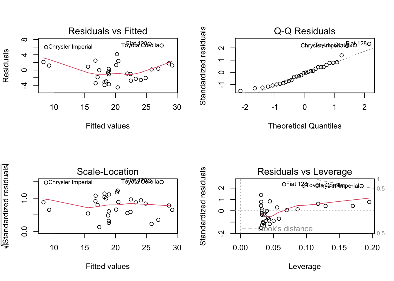

Interpretations:

Plot	Interpretation
Residuals vs Fitted	Checks the linearity assumption. Ideally, the residuals should be randomly scattered around 0, indicating that the model accurately captures the data’s trend.
Normal Q-Q	Assesses the normality of residuals. Points closely following the reference line suggest that residuals are normally distributed.
Scale-Location (or Spread-Location)	Evaluates homoscedasticity, which is the equal spread of residuals across all levels of the fitted values. A horizontal line with equally spread points indicates homoscedasticity.
Residuals vs Leverage	Identifies influential cases that might unduly affect the model’s predictions. Points far from the center suggest a high influence on the model estimate.

Your turn!

Please attempt these questions and write down your answers in the R Mardown workbook.
Run your codes in your workbook and compare your results with your deskmate.
Knit your workbook to publish a report in PDF or html.

Assignments

1. Linear Regression Model

Consider the regression model: \[ y_i= \alpha + \beta x_i + \epsilon_i \]

where \(\epsilon_i \sim \text{N}(0,\sigma^2)\) for \(i = 1,\ldots,n\). Here, y represents heights(in cm) and x represents weights(in kg).

Given a sample of heights and weights,

x<-c(82.62954, 66.73767, 83.29799, 82.72429, 74.14641, 54.60050, 60.71433,
     67.05280, 69.94233, 94.04653)
y<-c(202.5511,166.1328,194.1981,197.4564,181.9675,146.2233,160.5469, 166.2354,
     178.0746, 213.0961)

Find the maximum likelihood estimates for \(\alpha\) and \(\beta\) based on the given sample (Refer to Monday-1 Week 8 Lecture notes).
Plot a scatter plot of the sample and include the estimated regression line using the MLE of \(\alpha\) and \(\beta\). Providing the exact regression equation \(y=50+1.8*x+\epsilon\), where \(\epsilon \sim N(0,5^2)\), add this line into the plot.
Generate 100 simulations and calculate 100 values of \(\hat{\alpha}\) and \(\hat{\beta}\) using the regression \(y=50+1.8*x+\epsilon\), where \(\epsilon \sim N(0,5^2)\) and \(x \sim N(70,10^2)\). Calculate the variance of the MLE \((\hat{\alpha},\hat{\beta})\) using R and the formulas provided in Tuesday-1 Week 8 Lecture notes:

\[ \begin{aligned} & \operatorname{Var}(\hat{\beta})=\frac{\sigma^2}{\sum_{i=1}^n\left(x_i-\bar{x}\right)^2} \\ & \operatorname{Var}(\hat{\alpha})=\sigma^2\left(\frac{1}{n}+\frac{\bar{x}^2}{\sum_{i=1}^n\left(x_i-\bar{x}\right)^2}\right) \end{aligned} \]

Find the estimators’ variances as the sample size \(n\) increases, considering \(n = 100, 1000, 10000\).

2. Diagnostic Check

Consider women dataset which contains average heights and weights for American Women. Create a scatter plot of this data to examine the relationship between heights and weights. Is there evidence of a linear relationship?

 #access the dataset
data(women) #access the dataset

head(women)

  height weight
1     58    115
2     59    117
3     60    120
4     61    123
5     62    126
6     63    129

Fit a linear model to the data and perform a regression diagnostics check, including standard linear model diagnostics.