# Simulating a Poisson-distributed sample
set.seed(123)
theta_true <- 4
n_samples <- 10
sample_data <- rpois(n_samples, theta_true)

sample_data
[1] 3 6 3 6 7 1 4 7 4 4Statistical Estimations
\(\hat{p} = \frac{1}{n}\sum_{i=1}^{n}x_i\), where \(x_i\) are the observed values.
\(\hat{p} = \frac{\bar{x}}{n}\), where \(\bar{x}\) is the sample mean.
\(\hat{\theta} = \bar{x}\), where \(\bar{x}\) is the sample mean.
\(\hat{\mu} = \bar{x}\) and \(\hat{\sigma}^2 = \frac{1}{n}\sum_{i=1}^{n}(x_i - \bar{x})^2\).
We will find the MLE of a Poisson sample, plot the log-likelihood function, find its maximum, and compare with the theoretical value. Recall that the Possion distribution:
\[ P(X=x)=\exp^{-\theta}\frac{\theta^x}{x!} \]
# Simulating a Poisson-distributed sample
set.seed(123)
theta_true <- 4
n_samples <- 10
sample_data <- rpois(n_samples, theta_true)
sample_data [1] 3 6 3 6 7 1 4 7 4 4The log-likelihood function for Possion distribution:
\[ \begin{align} l(\theta;\vec{x}) &= -n\theta + \ln{\theta}\cdot \left(\sum_{i=1}^n x_i\right) - \underbrace{\ln \left(\prod_{i=1}^n x_i!\right)}_{\text{constant in }\theta} \\ \end{align} \]
log_likelihood <- function(theta, data) {
  sum(data)*log(theta)-length(data)*theta
}

theta_seq <- seq(1, 8, by = 0.1)
ll_values <- sapply(theta_seq, log_likelihood, data = sample_data)

plot(theta_seq, ll_values, type = "l", main = "Log-Likelihood Function", xlab = "theta", ylab = "Log-Likelihood")

MLE <- mean(sample_data)
abline(v = MLE)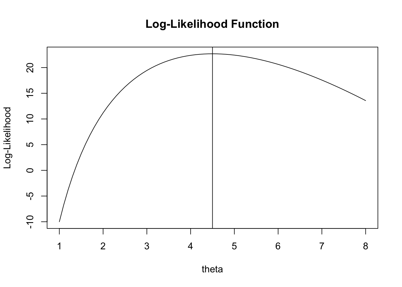
opt1 <-optimize(f=log_likelihood, data = sample_data, interval=c(0,7),maximum=TRUE)

optimiser <- opt1$maximum

cat("The MLE for theta is:", MLE, "\n")
The MLE for theta is: 4.5 cat("The optimiser for the log-likelihood is", optimiser, "\n")The optimiser for the log-likelihood is 4.499999 Suppose we observe data \(\vec{x}=(1,0,0,1,0,1,0,0,1,1)\) where each element \(X_i\) follows a Bernoulli distribution with an unknown success probability \(p\).
Find the likelihood function \(L(p;\vec{x})\) which represents the joint pdf function of \(p\) given the observed data \(\vec{x}\) and define it as a function in R. Calculate the value of this function at \(p=0.1\).
Plot the likelihood function for \(p\in[0,1]\) and use the optimize() function to find the point that maximizes \(L(p;\vec{x})\). Add a vertical line to the plot to indicate this maximum point.
Calculate the log-likelihood function \(l(p;\vec{x})\) and define this function in R. Plot the log-likelihood function. Verify that \(p=0.5\) maximizes the log-likelihood function by setting its first derivative equal to zero and ensuring that the second derivative is negative.
Given that \(X \sim \text{Bin}(n,p)\) and observed that \(n=10\) and \(x=3\).
Define the likelihood function in R and calculate it at \(p=0.1\).
Plot the likelihood function for \(p\in[0,1]\) and calculate the maximum likelihood estimate. Add a vertical line to the plot to indicate this maximum point.
Given the heights(in cm) of a random sample of 20 students:
182, 154, 147, 150, 164, 177, 169, 173, 160, 173, 170, 160, 178, 175, 154, 179, 168, 188, 172, 162
We assume that the heights of students follow a normal distribution with unknown mean \(\mu\) and standard deviation \(\sigma\).
Determine the maximum likelihood estimates of \(\mu\) and \(\sigma\) based on the given sample.
Calculate the log-likelihood of these height estimates.